Appendix F: Miscellaneous
AWG2021 User Manual
FĆ3
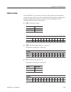
Sampling Theorem
When the signal is continuous and the highest frequency component of the signal
is f
0, sampling with Te1/2f0 loses none of the data contained in the signal. T is
the sampling interval. This theorem is well known as the sampling theorem. If
data is created to meet this theorem, the necessary signal can be obtained.
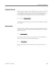
X(t) +
ȍ
R
n+–R
X(nt)
sin
NJ
(2pńT)(t–nTń2)
Nj
(2pńT)(t–nTń2)
A continuous analog signal x(t) can be reproduced from the digital data with the
above equation.
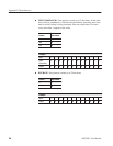
Differentiation
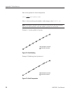
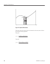
The diff() function calculates the central deviation as the differential value. The
equation below expresses the central deviation when the function f(x) is given at
even intervals of nx.
fȀ(x) [
f (x ) Dx)–f (x–Dx)
(2 Dx)
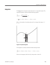
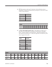
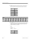
In actual practice, when function f(x)is expressed by n values, the differential
value f’(x
i) at point xi is given by the following equation.
fȀ(x
i
) [ n
{
f (x
i)1
)–f(x
i–1
)
}
2
Here, n is the number of waveform points and i is an integer in the range, i = 1,
2, ..., n.


